Gephi is a free graph analysis and visualisation tool developed over the Netbeans platform for Java. It supports computing statistics over graphs, applying algorithms to analyse and to visualise the graphs, and to apply filters and queries over the graphs, all using an intuitive graphical-user interface (GUI). It has become very popular today due to its strong capabilities and support by the user community. We will demonstrate in this article how to use it to visualise a proximity graph for the data lake.
A proximity graph is one where nodes represent datasets stored in the data lake and edges represent their overall computed similarity (or in other words, "proximity". This can be computed using our proposed techniques here). Here is a sequence of steps for constructing such graphs:
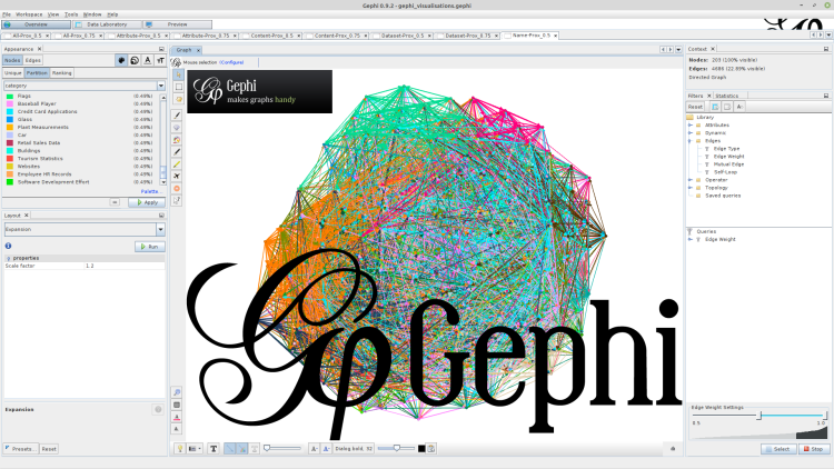
0- Create an empty Gephi project.
1- Import the nodes and edges tables into a new workspace. They should be stored as comma-separated values (CSV files) where the nodes table has the columns "id":integer as a unique identifier, "label":string as a label for the nodes (here we can use the dataset names or filenames), in addition to any extra columns with further information. For the edges table, it should include "source" and "target" columns having the "id" of the nodes they represent for an edge, "weight":numeric to give a weight to the edge (i.e., how strong the relationship or connection is? In our case, this should represent similarity between datasets similar to our paper here), and "label" to indicate a label for the edge.
To import those nodes and edges tables, use the following: File --> Import spreadsheet ... --> (select the CSV file from the file browser interface).
Gephi automatically identifies if the CSV represents nodes or edges based on the column names they store. If a CSV file has "id" and "label" columns only then it is a nodes table, and if it includes "source" and "target" columns then it represents edges.
2- Apply Nodes partitioning to colour the nodes using any column in the nodes table.
This is done from the top left panel as follows: Appearance --> Nodes --> (select colour icon from top right buttons in the panel) --> Partition --> (select column name from nodes table) --> click Apply.
3- You can filter the edges by weight (make sure that the edges table has a "weight" column, and it must have the same exact name to work!) in the graph using the "filters" and "queries" panels in the right panels of the workspace.
This is done as follows: Filters --> Edges --> (drag-and-drop "Edge Weight" to the "Queries" panel below the filters panel) --> (select the minimum and maximum values for the edges weight using the value selector that appears below the "Queries" panel in the "Edge Weight Settings" panel that now appears.)
4- You can also reorder the nodes and edges visualised in the graph in the middle view by applying famous algorithms like "ForceAtlas".
To do so, in the "Layout" panel in the bottom-left panel, select "ForceAtlas" from the drop-down menu, leave the default parameters selected, then press the "run" button. Leave the algorithm to run for a few seconds as the nodes and edges get repositioned live as the algorithm is running. "stop" the algorithm by pressing the button when the nodes and edges stop moving in the middle view or when satisfied with the current positioning.
5- After the "ForceAtlas 2" algorithm is done, make sure to apply a "nonoverlap" from the drop-down menu in "Layout" panel in order to separate overlapping nodes and edges, and also to apply "Expansion" and "Contraction" layout steps from the same drop-down menu in order to spread or compress the graph view accordingly.
This way, we are able to visualise any graphs which have nodes representing objects and edges representing a relationship (for instance, similarity) with specific strength (or edge weights in Gephi's terminology). This is the basis for constructing proximity graphs over data lakes using Gephi.